Business Area
Bike-sharing and membership marketing
Data Analytics Case Study
Understanding how annual members and casual riders use Cyclistic bicycles differently
Python * Pandas * Data Cleaning * Exploratory Data Analysis * Matplotlib * Data Storytelling
This project analyzes Cyclistic bike-share trip data to identify meaningful differences between annual members and casual riders. The goal is to support marketing strategies that could encourage casual riders to become annual members.
Bike-sharing and membership marketing
Annual members and casual riders
Identify opportunities to convert casual riders into annual members
Python, Pandas and Matplotlib
Cyclistic offers bicycles through annual memberships and single-ride or day-pass options. The company wants to understand how annual members and casual riders use the service differently.
Understanding these behavioural differences can help the marketing team design campaigns that are more relevant to casual riders and encourage them to purchase annual memberships.
How do annual members and casual riders use Cyclistic bicycles differently?
The analysis uses historical bike-share trip data containing individual ride records. Each row represents one bicycle trip and includes rider type, bicycle type, start time, end time and station information.
Member and casual
Ride ID, rider type, bicycle type, start time, end time and station information
Ride length, weekday and additional time-based variables
Descriptive and exploratory data analysis
The analysis followed a structured approach from asking the right question to delivering actionable recommendations.
Defined the business problem and main analytical question.
Imported and reviewed the bike-share datasets.
Cleaned the data and created fields needed for analysis.
Compared ride frequency and duration between members and casual riders.
Created charts and communicated the main findings.
Developed marketing recommendations from the evidence.
This section connects the Python code to its analytical purpose, output and business value. Click each step to explore the complete workflow.
The Python environment was prepared by importing the libraries needed for data manipulation, numerical calculations and visualisation.
import pandas as pd
import numpy as np
import matplotlib.pyplot as plt
import seaborn as sns
pd.set_option('display.max_columns', None)Import the tools needed to load, clean, transform, analyse and visualise the Cyclistic trip data.
Pandas manages the dataset, NumPy supports numerical operations, and Matplotlib and Seaborn create charts.
These libraries provide the analytical foundation needed to transform raw trip records into meaningful business insights.

Multiple monthly CSV files were loaded and combined into one complete DataFrame for the analysis period.
import glob

files = sorted(
    glob.glob(
        "/kaggle/input/datasets/ashwinraphel/"
        "cycle-new-data-set/2025*.csv"
    )
)

df_list = []

for file in files:
    temp_df = pd.read_csv(file)
    df_list.append(temp_df)

df = pd.concat(df_list, ignore_index=True)

print(df.shape)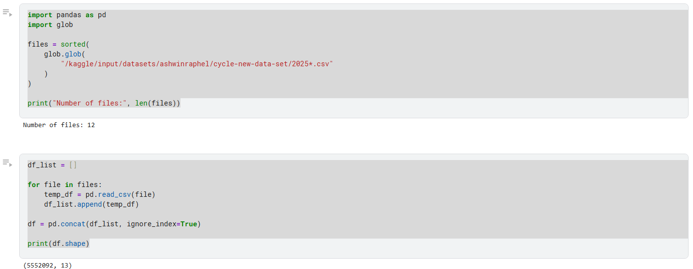
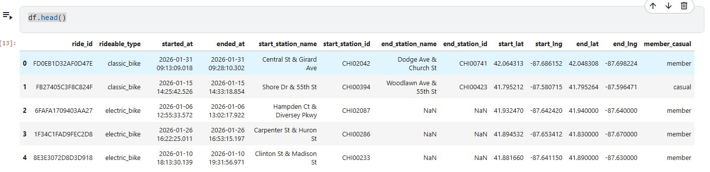
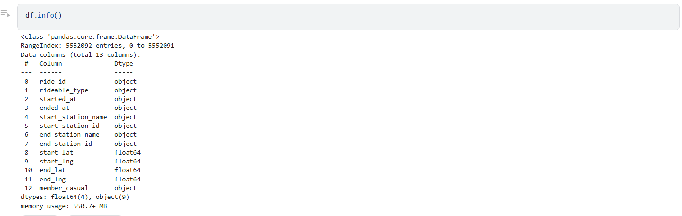
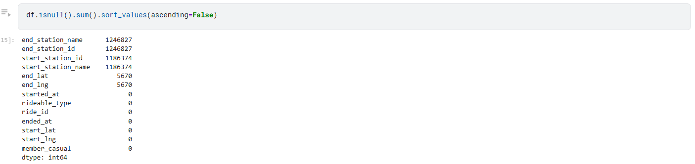
The dataset was inspected before cleaning to understand its structure, quality and overall characteristics.
df.shape
df.head()
df.info()
df.isnull().sum().sort_values(ascending=False)The dataset size was checked to confirm the total number of rows and columns.
Column names were reviewed to understand the available dataset fields.
Data types were inspected to confirm that each column used an appropriate format.
Missing values were identified before beginning the cleaning process.
Sample records were reviewed to understand the dataset content and structure.
The data was cleaned to ensure that comparisons and visualisations were based on valid and consistent records.
df['started_at'] = pd.to_datetime(
    df['started_at']
)

df['ended_at'] = pd.to_datetime(
    df['ended_at']
)

df['ride_length'] = (
    df['ended_at'] - df['started_at']
).dt.total_seconds() / 60

df = df[df['ride_length'] > 0]
df = df[df['ride_length'] <= 1440]Start and end times were converted from text into datetime values.
Ride duration was calculated in minutes.
Negative, zero-length and rides longer than 24 hours were removed.
Missing station records were retained because they did not affect the main business question.
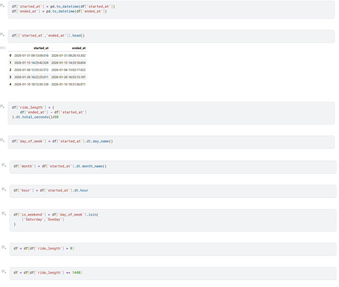

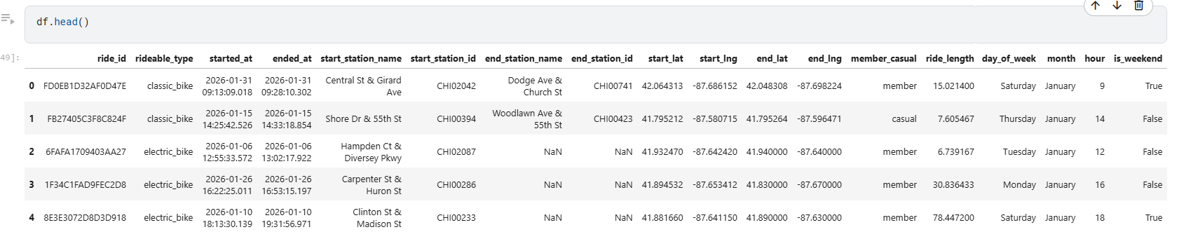
New variables were created from the timestamps to support deeper behavioural comparisons.
df['ride_length'] = (
    df['ended_at'] - df['started_at']
).dt.total_seconds() / 60

df['day_of_week'] = (
    df['started_at'].dt.day_name()
)

df['month'] = (
    df['started_at'].dt.month_name()
)

df['hour'] = (
    df['started_at'].dt.hour
)

df['is_weekend'] = (
    df['day_of_week'].isin(
        ['Saturday', 'Sunday']
    )
)Measures trip duration in minutes.
Supports comparisons across different weekdays.
Supports seasonal and monthly trend analysis.
Supports time-of-day usage analysis.
Distinguishes weekday rides from weekend rides.
Rider groups were compared across ride frequency, duration, weekday activity, monthly trends and bike preferences.
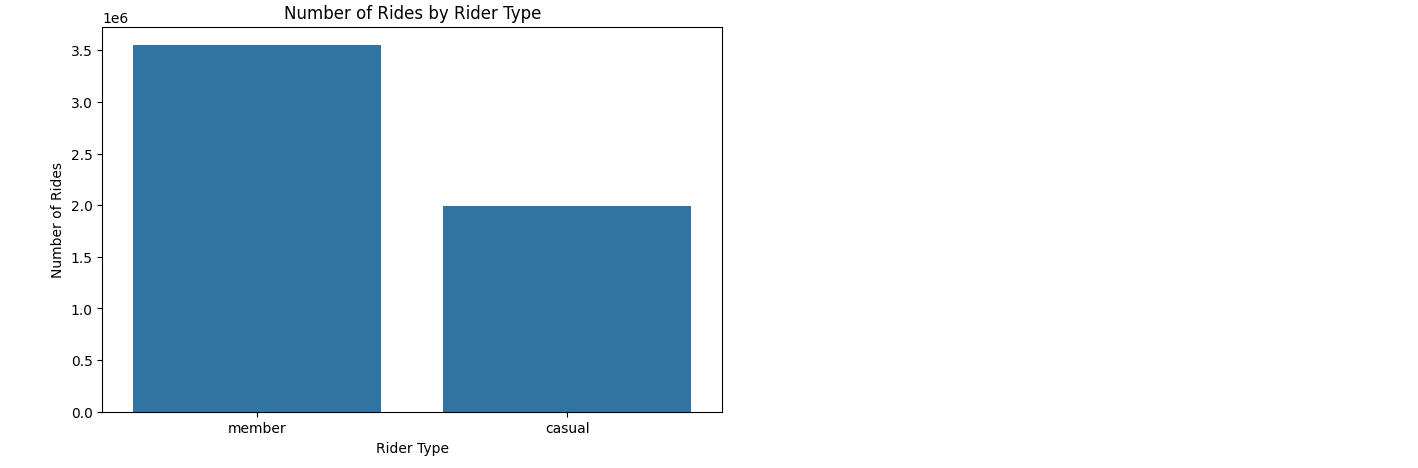
Members completed approximately 3.55 million rides, compared with approximately 2 million casual rides.
Members demonstrate more frequent usage and form Cyclistic's core customer group.
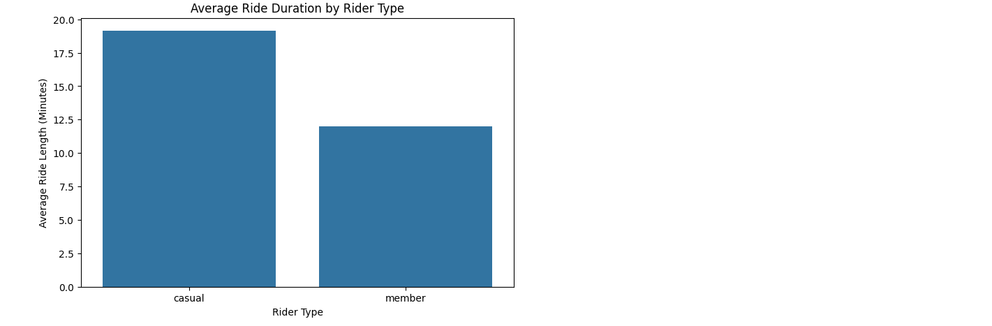
Casual rides averaged around 19.1 minutes, compared with 12 minutes for members.
Casual riders appear more likely to use bikes for recreation and leisure.
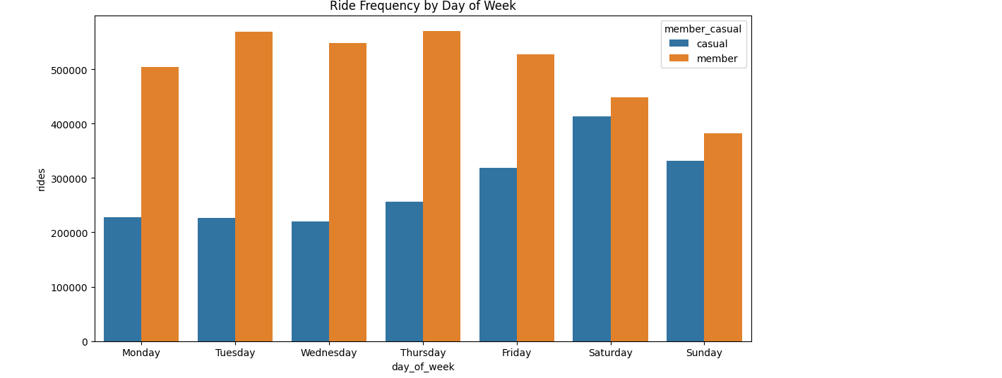
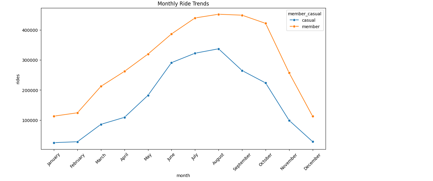
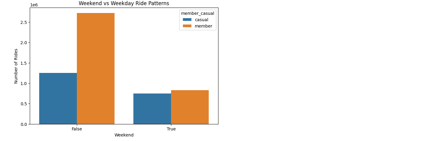
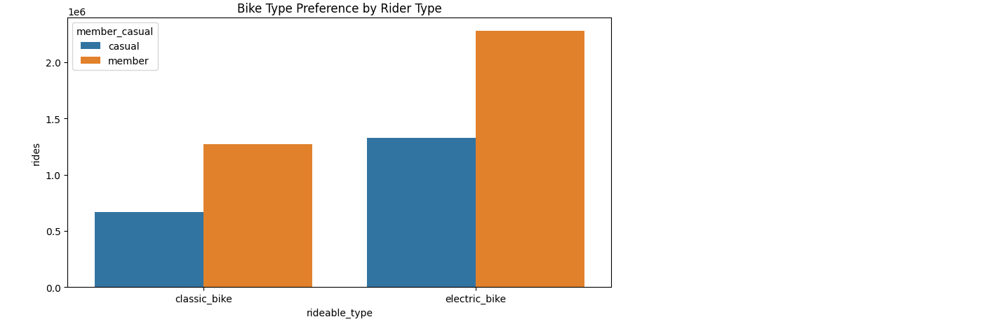
Each visualization connects the Python analysis to a clear observation and a practical business insight.
Compares the total number of rides completed by annual members and casual riders.
Shows how average trip length differs between members and casual riders.
Identifies how rider activity changes across the days of the week.
Highlights seasonal demand patterns and monthly changes in ride activity.
Compares ride activity on working days and weekends to reveal commuting and leisure patterns.
Compares the bicycle types selected by members and casual riders.
The analysis revealed important differences in how members and casual riders use Cyclistic bicycles.
Casual riders had a higher average ride duration than annual members.
Annual members used the service more frequently, indicating regular and repeated usage.
Members appear more likely to use bicycles for routine transport, while casual riders appear more likely to ride for leisure.
Differences by day and time can help Cyclistic target campaigns more effectively.
Based on the rider behaviour analysis, the following recommendations can help Cyclistic increase annual memberships and improve customer engagement.
Target casual riders during weekends and periods of high recreational usage, when they are most engaged with the service.
Demonstrate how an annual membership can reduce long-term riding costs for frequent casual riders through targeted pricing messages.
Encourage conversion by providing limited-time discounts, free trial memberships, or promotional offers to riders with repeated casual usage.
Personalize marketing campaigns using rider behaviour, preferred riding periods, seasonal demand, and bicycle usage patterns to improve conversion rates.
The complete notebook includes the Python code, data preparation steps, calculations, visualizations and detailed analysis used in this case study.